An outlier is an observation which deviates so much from the other observations as to arouse suspicions that it was generated by a different mechanism.
D.M. Hawkins (1980) Identification of OutliersAnomaly detection is a powerful set of techniques that belong in every data scientists toolset.
Anomaly detection is the identification of unusual data points that deviate significantly from expected patterns or normal behavior.
These unusual observations can indicate:
Understanding your domain is crucial for effective anomaly detection. The definition of “normal” depends entirely on context - what’s anomalous in financial transactions differs from what’s anomalous in network traffic or medical data.
An anomaly detector is an algorithm that automatically identifies records as anomalies based on statistical, distance-based, or machine learning techniques.
The choice of detector depends on your data characteristics, domain knowledge, computational constraints, and interpretability requirements.
Resources to learn anomaly detection:
Anomaly detection enables you to:
Anomaly detection methods apply across many domains - the same statistical methods that detect credit card fraud can find manufacturing defects or identify unusual patient symptoms.
Applications of anomaly detection include:
If the outliers are only outliers because of noise, they are weak outliers. Strong outliers are outliers because they are generated by different data generating processes.
Internal outliers are less common than extreme values. They appear only in multimodal distributions or distributions with gaps.
Internal outliers can be detected by the following algorithms, which are more flexible to unusual distributions:
Global outliers are unusual when compared to the entire dataset. These points are far from all other data points and would be considered anomalies regardless of local context.
Local outliers are unusual only within their local neighborhood, but may appear normal when viewed globally. A point might be close to one cluster but far from the specific cluster it should belong to.
Local outliers are also known as in-distribution anomalies, while global outliers are out-of-distribution anomalies.
Masking occurs when the presence of outliers causes other outliers to not be detected. This happens because extreme outliers can shift statistical measures (like mean and standard deviation) so much that other outliers appear normal by comparison.
import numpy as np
import matplotlib.pyplot as plt
from scipy import stats

# Generate normal data with two types of outliers
np.random.seed(42)
normal_data = np.random.normal(0, 1, 100)
moderate_outliers = [3.5, 3.7]  # These should be detected
extreme_outliers = [15, 16]     # These mask the moderate ones

data = np.concatenate([normal_data, moderate_outliers, extreme_outliers])

# Z-score detection (affected by masking)
z_scores = np.abs(stats.zscore(data))
outliers_zscore = data[z_scores > 2]

# Robust detection using MAD
mad = np.median(np.abs(data - np.median(data)))
modified_z_scores = 0.6745 * (data - np.median(data)) / mad
outliers_mad = data[np.abs(modified_z_scores) > 2]

print(f"Z-score outliers: {outliers_zscore}")
print(f"MAD outliers: {outliers_mad}")
Z-score outliers: [15. 16.]
MAD outliers: [-1.91328024 -1.72491783 1.85227818 -1.95967012 -1.76304016 -2.6197451
-1.98756891 3.5 3.7 15. 16. ]Moderate outliers [3.5, 3.7] missed by Z-score due to masking from extreme outliers [15, 16]

Swamping occurs when the presence of outliers causes normal points to be incorrectly identified as outliers. This typically happens when outliers inflate the variance, making the detection threshold too sensitive.
import numpy as np
import matplotlib.pyplot as plt
from scipy import stats

# Generate clustered data with one extreme outlier
np.random.seed(42)
cluster1 = np.random.normal(0, 0.5, 50)
cluster2 = np.random.normal(5, 0.5, 50)
extreme_outlier = [20]  # This will cause swamping

data = np.concatenate([cluster1, cluster2, extreme_outlier])

# Z-score detection (affected by swamping)
z_scores = np.abs(stats.zscore(data))
outliers_zscore = data[z_scores > 2]

# Robust detection using median and MAD
median_val = np.median(data)
mad = np.median(np.abs(data - median_val))
modified_z_scores = 0.6745 * (data - median_val) / mad
outliers_mad = data[np.abs(modified_z_scores) > 2]

print(f"Z-score outliers (swamping): {len(outliers_zscore)} points")
print(f"MAD outliers (robust): {len(outliers_mad)} points")
Z-score outliers (swamping): 1 points
MAD outliers (robust): 1 points
Z-score detected: [20.]
MAD detected: [20.]The extreme outlier 20 inflated variance, causing normal points to be flagged as outliers.

An anomaly label is a binary classification of whether a record is an anomaly or not. Generating a label is often done with a score and a threshold.
An anomaly score is a continuous value that indicates how abnormal a record is. Example of scores include a z score, a distance from a cluster, or a density estimate.
Scores can be combined and ranked, although care is needed when combining scores on different scales. Scores can be combined with the sum, maximum or sum of squares.
Univariate outlier detection uses a single feature to find unusual values. The scores created with univariate anomaly detection can be combined for all features in a row, to generate an estimate for the entire row.
Univariate outiler detection has one source of unusualness - unusual because of the single feature. A univariate outlier detection model cannot understand the relationships between features.
Multivariate outlier detection uses many features, and can find unusual combinations of unusual values alongside just finding unusual values.
Multivariate outlier detection has two sources of unusualness - unusual because of the single feature and/or unusual when combined with other features.
The curse of dimensionality refers to the problems that arise when working with high-dimensional data.
Very few outliers require many features to detect them. Some outliers can only be detected in high dimensions.
For outlier detection, high dimensions cause the following issues:
One common way to detect anomalies with categorical variables is with counts. Anomalies can then be detected by thresholds on the counts.
Can set a threshold on a cumulative count. Here you would set a record to an anomaly based on the cumulative count of all values of that column, stopping where the total is equal to a threshold of 1% (for example).
You can also do outlier detection on the counts - for example using MAD or z score on the counts.
Marginal probabilities detect anomalies in categorical features by identifying values with unusually low probability of occurrence. This method calculates the probability of each category value and flags records containing rare combinations.
The marginal probabilities method is particularly effective for:
Basic marginal probability calculation:
import pandas as pd
import numpy as np

# Sample categorical data
data = pd.DataFrame({
    'department': ['Sales', 'Sales', 'Engineering', 'Engineering', 'Marketing', 'Legal'],
    'location': ['NYC', 'NYC', 'SF', 'SF', 'NYC', 'Remote'],
    'level': ['Junior', 'Senior', 'Senior', 'Senior', 'Senior', 'Partner']
})

# Calculate marginal probabilities for each feature
dept_probs = data['department'].value_counts(normalize=True)
location_probs = data['location'].value_counts(normalize=True)
level_probs = data['level'].value_counts(normalize=True)

print("Department probabilities:")
print(dept_probs)
print("\nLocation probabilities:")
print(location_probs)
print("\nLevel probabilities:")
print(level_probs)
Department probabilities:
department
Sales 0.333333
Engineering 0.333333
Marketing 0.166667
Legal 0.166667
Location probabilities:
location
NYC 0.5
SF 0.333333
Remote 0.166667
Level probabilities:
level
Senior 0.666667
Junior 0.166667
Partner 0.166667Detecting anomalies using probability thresholds:
# Set threshold for rare categories (probability < 0.2)
threshold = 0.2

# Find records with rare categorical values
anomalies = []
for idx, row in data.iterrows():
    dept_prob = dept_probs[row['department']]
    loc_prob = location_probs[row['location']]
    level_prob = level_probs[row['level']]

    # Flag if any category has probability below threshold
    if dept_prob < threshold or loc_prob < threshold or level_prob < threshold:
        anomalies.append({
            'index': idx,
            'department': row['department'],
            'location': row['location'],
            'level': row['level'],
            'dept_prob': dept_prob,
            'loc_prob': loc_prob,
            'level_prob': level_prob
        })

print(f"Found {len(anomalies)} anomalous records:")
for anomaly in anomalies:
    print(f"Row {anomaly['index']}: {anomaly['department']}, {anomaly['location']}, {anomaly['level']}")
    print(f"  Probabilities: dept={anomaly['dept_prob']:.3f}, loc={anomaly['loc_prob']:.3f}, level={anomaly['level_prob']:.3f}")
Found 3 anomalous records:
Row 4: Marketing, NYC, Senior
Probabilities: dept=0.167, loc=0.500, level=0.667
Row 5: Legal, Remote, Partner
Probabilities: dept=0.167, loc=0.167, level=0.167
Row 0: Sales, NYC, Junior
Probabilities: dept=0.333, loc=0.500, level=0.167Combined probability scoring:
# Calculate combined probability score for each record
data['combined_prob'] = data.apply(lambda row:
    dept_probs[row['department']] *
    location_probs[row['location']] *
    level_probs[row['level']], axis=1)

# Sort by combined probability (lowest = most anomalous)
data_sorted = data.sort_values('combined_prob')
print("Records sorted by combined probability (most anomalous first):")
print(data_sorted[['department', 'location', 'level', 'combined_prob']])
Records sorted by combined probability (most anomalous first):
department location level combined_prob
5 Legal Remote Partner 0.004630
0 Sales NYC Junior 0.027778
4 Marketing NYC Senior 0.055556
1 Sales NYC Senior 0.111111
2 Engineering SF Senior 0.148148
3 Engineering SF Senior 0.148148Visualization is crucial for understanding your data and validating anomaly detection results. Different chart types work best for different data combinations.
Histogram: Shows the distribution and identifies gaps or unusual peaks
data = [1, 2, 3, 4, 5, 100]  # 100 is an outlier
plt.hist(data, bins=10, alpha=0.7, edgecolor='black')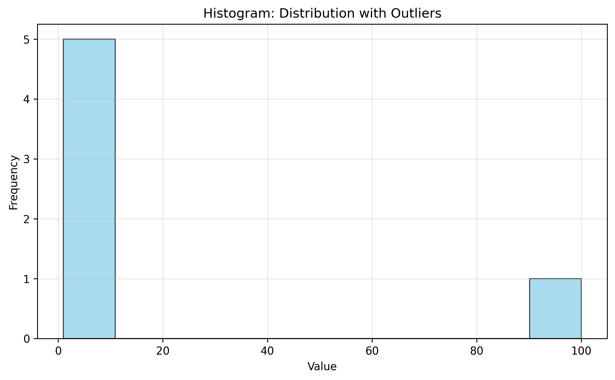
Kernel Density Estimation (KDE): Smooth density curves that highlight low-density regions
sns.histplot(data, kde=True, alpha=0.7)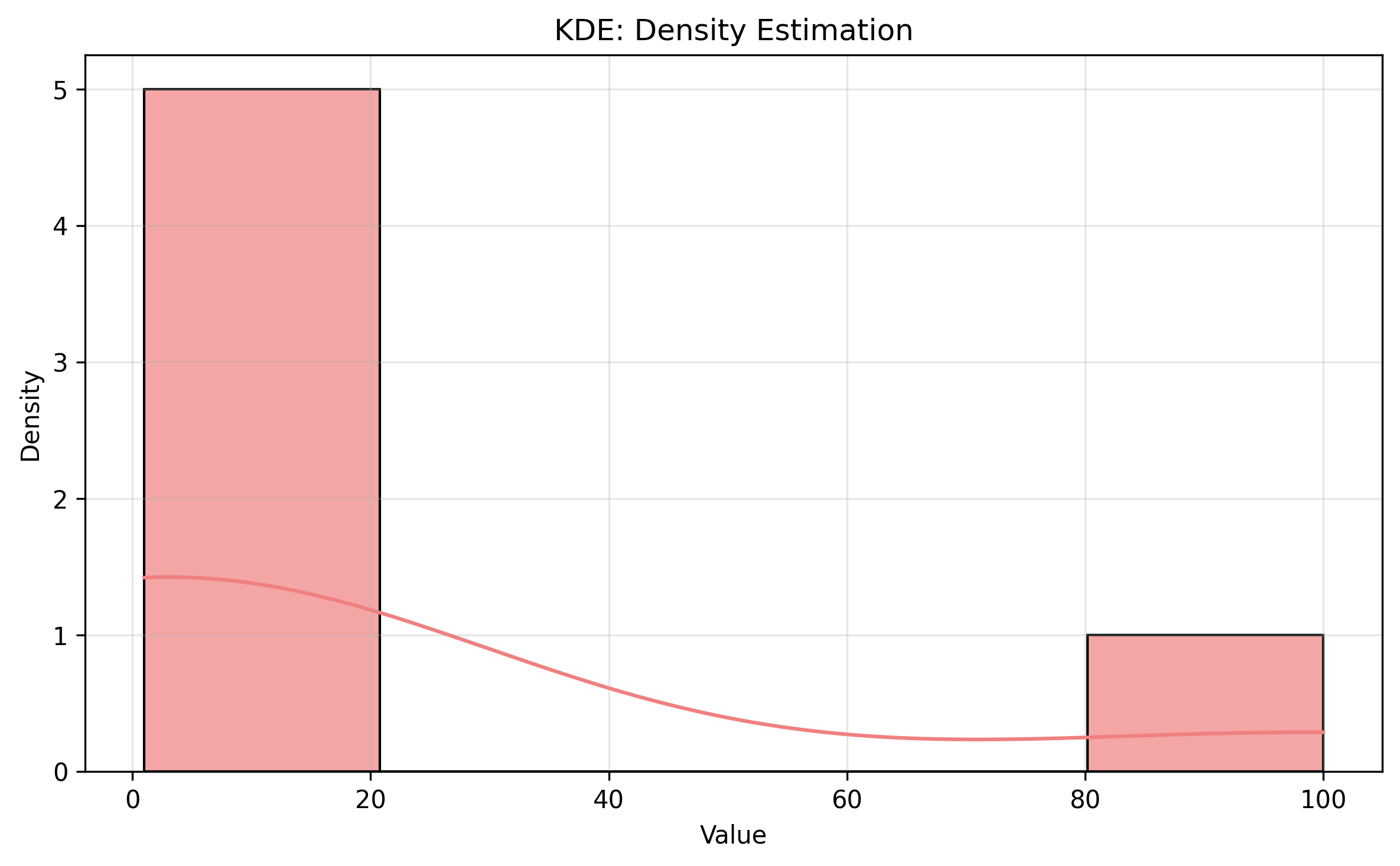
Boxplot: Identifies outliers using quartiles and IQR
plt.boxplot(data) # Points beyond whiskers are outliers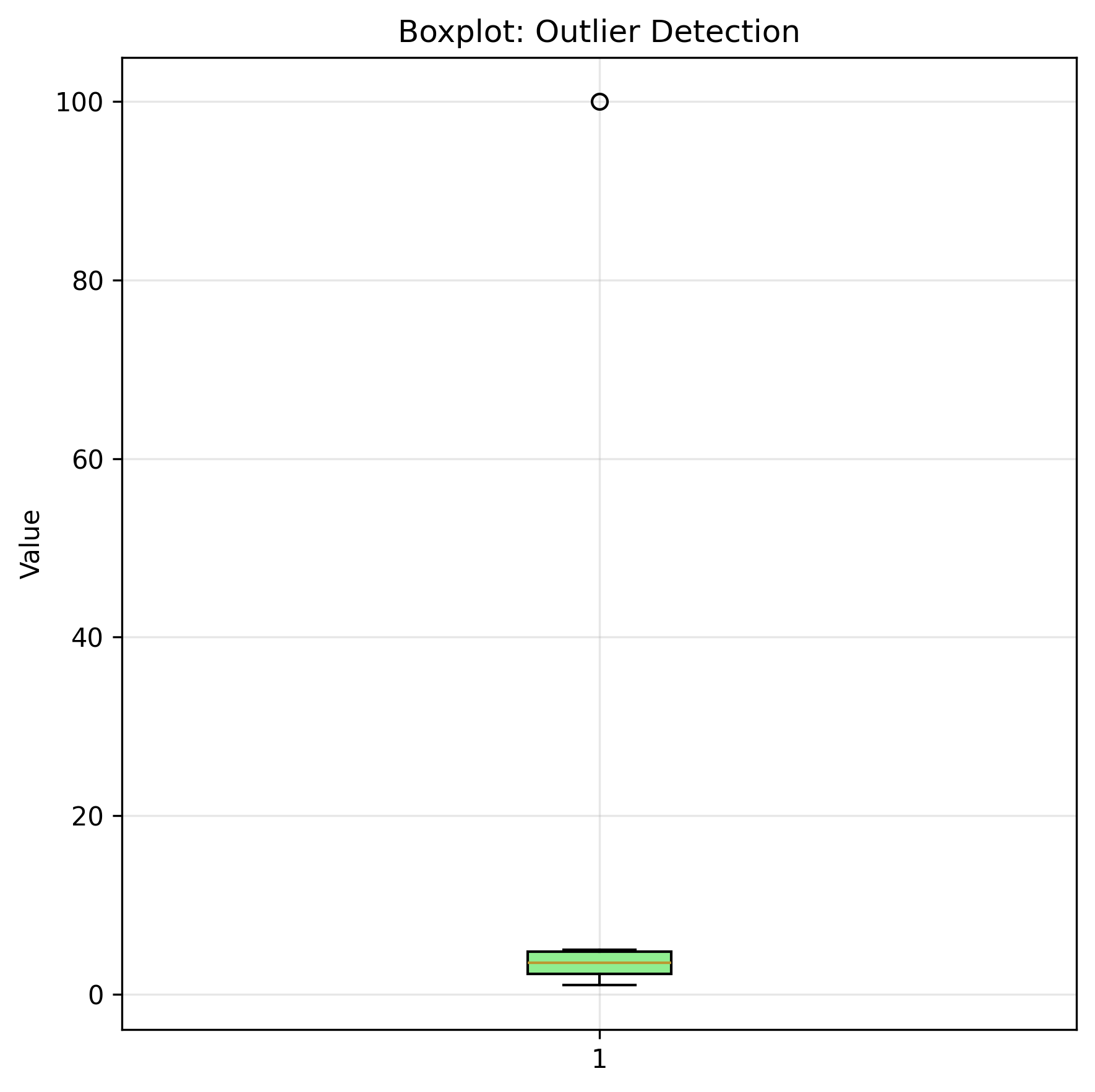
Scatterplot: Reveals outlying points and clusters in two numeric variables
x = [1, 2, 3, 4, 10]
y = [1, 2, 3, 4, 10]  # (10, 10) is an outlier
plt.scatter(x, y)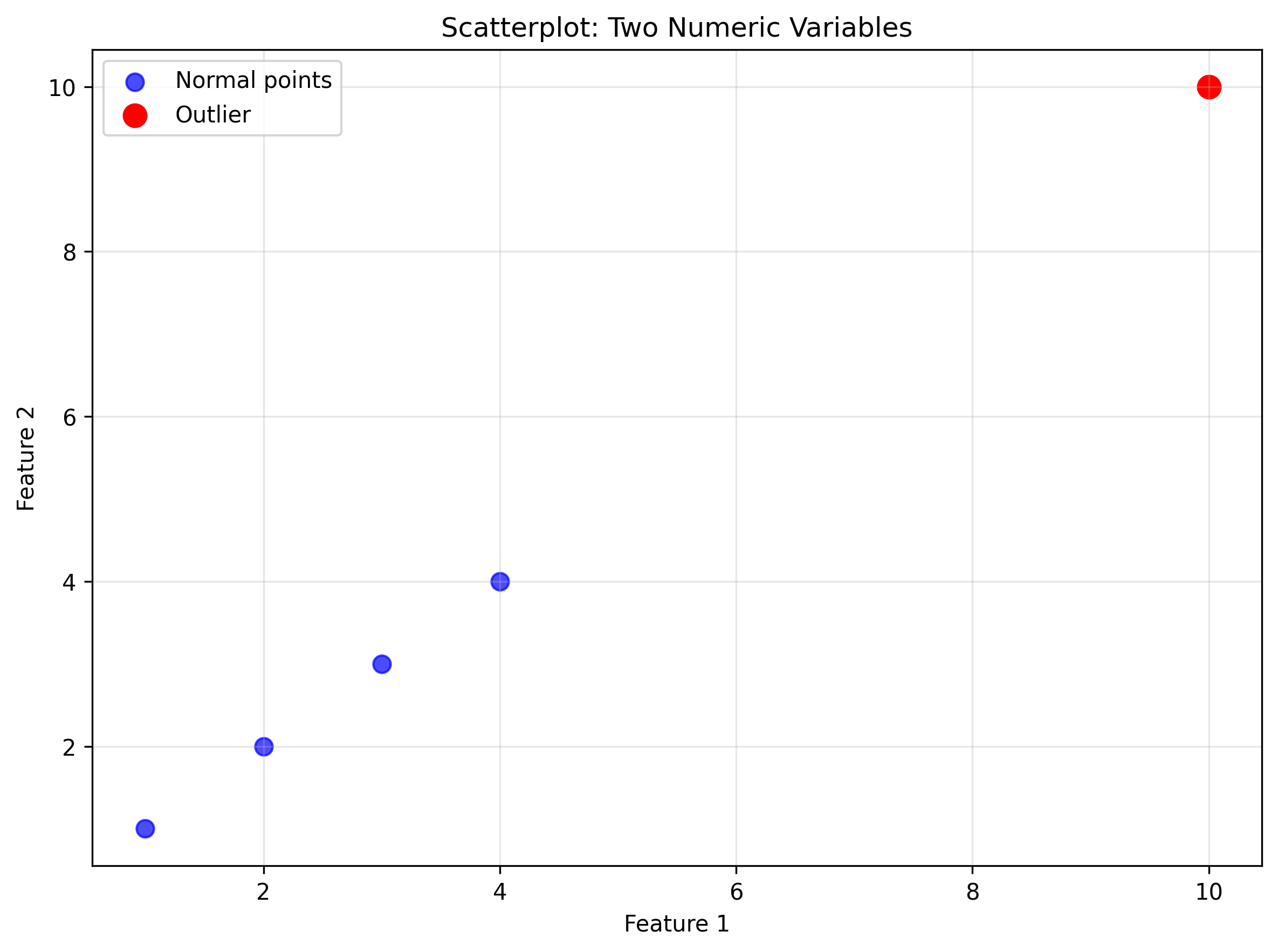
Heatmap: Shows frequency patterns between two categorical variables
df = pd.DataFrame({'cat1': ['A', 'A', 'B'], 'cat2': ['X', 'Y', 'Z']})
heatmap_data = pd.crosstab(df['cat1'], df['cat2'])
sns.heatmap(heatmap_data, annot=True)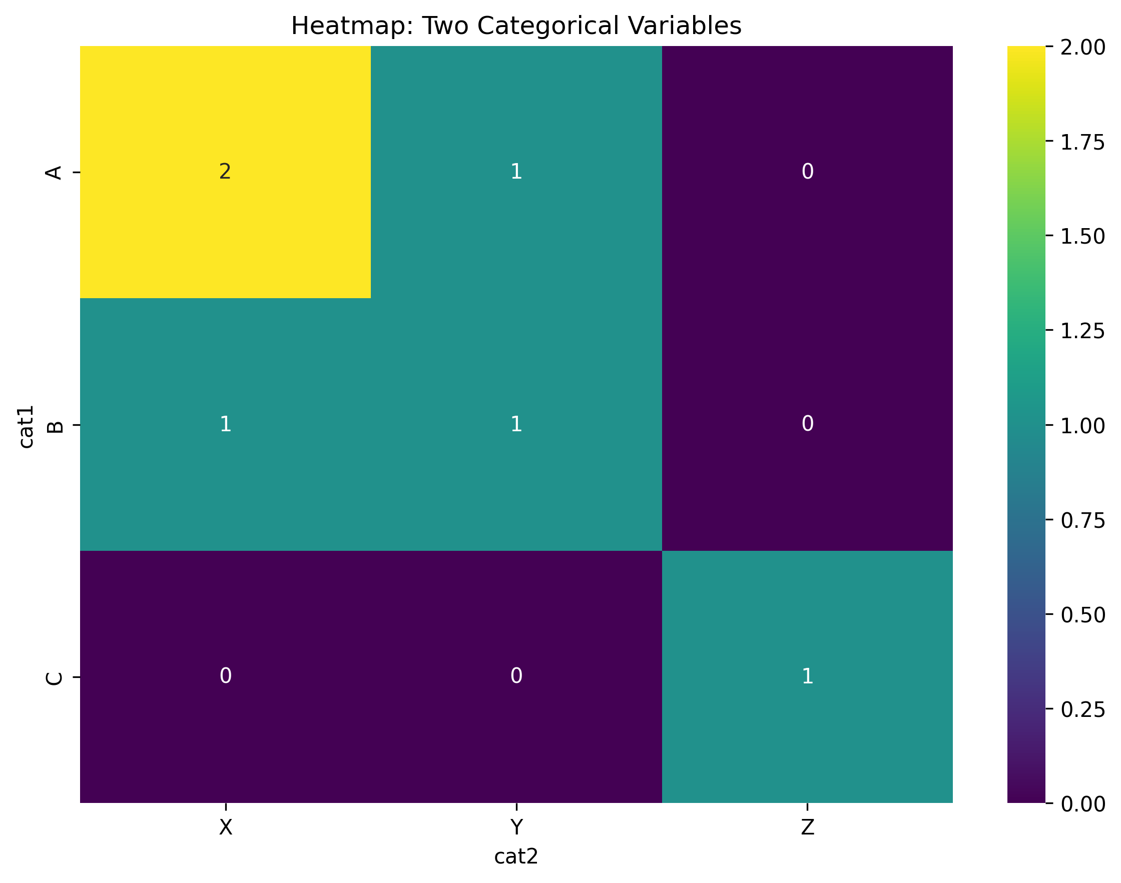
Boxplot by category: Identifies outliers within categorical groups
data_by_group = [[1, 2, 3, 4], [10, 11, 12, 100]]  # 100 is outlier in group 2
plt.boxplot(data_by_group, tick_labels=['Group A', 'Group B'])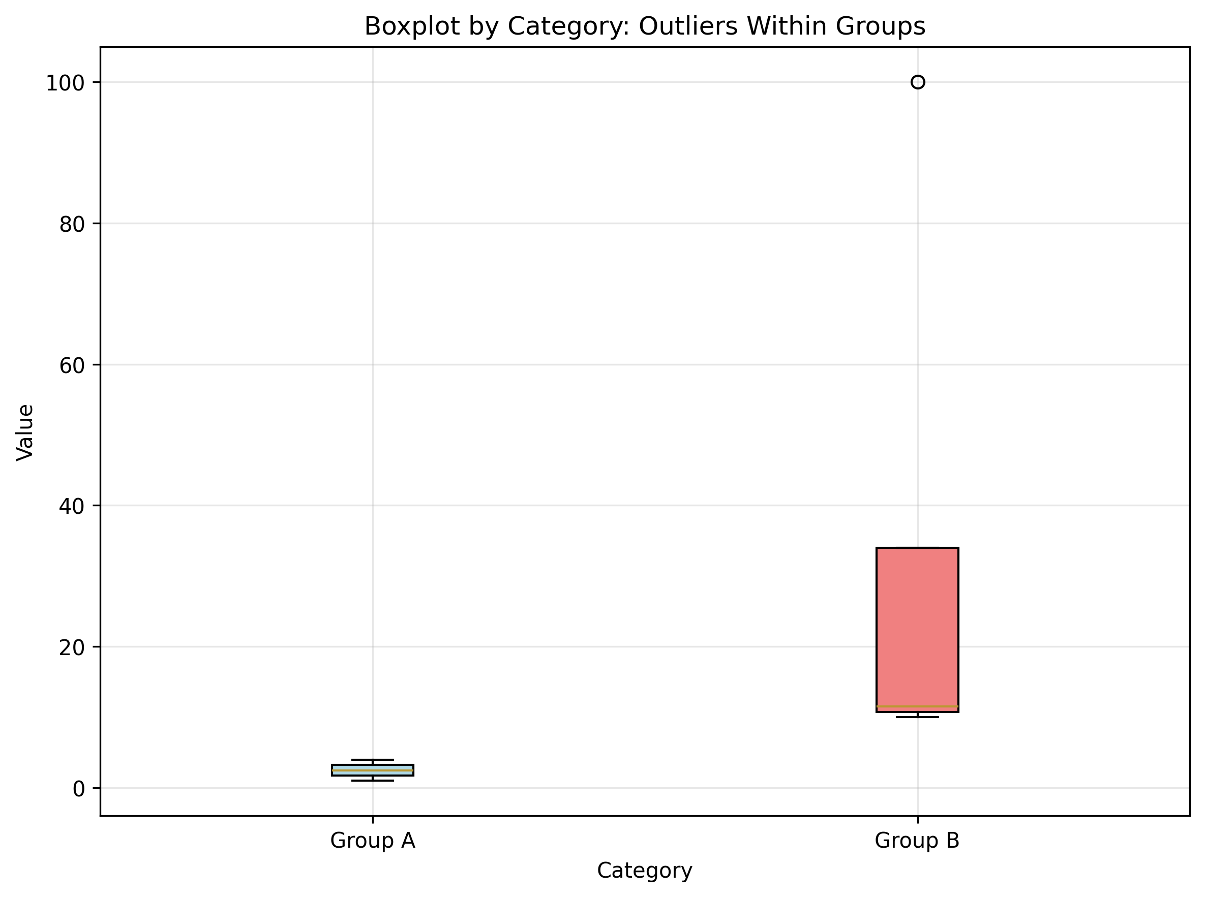
Z-score visualization: Color-codes points by their statistical outlier scores
z_scores = np.abs(stats.zscore(data))
plt.scatter(range(len(data)), data, c=z_scores, cmap='Reds')
plt.colorbar(label='|Z-score|')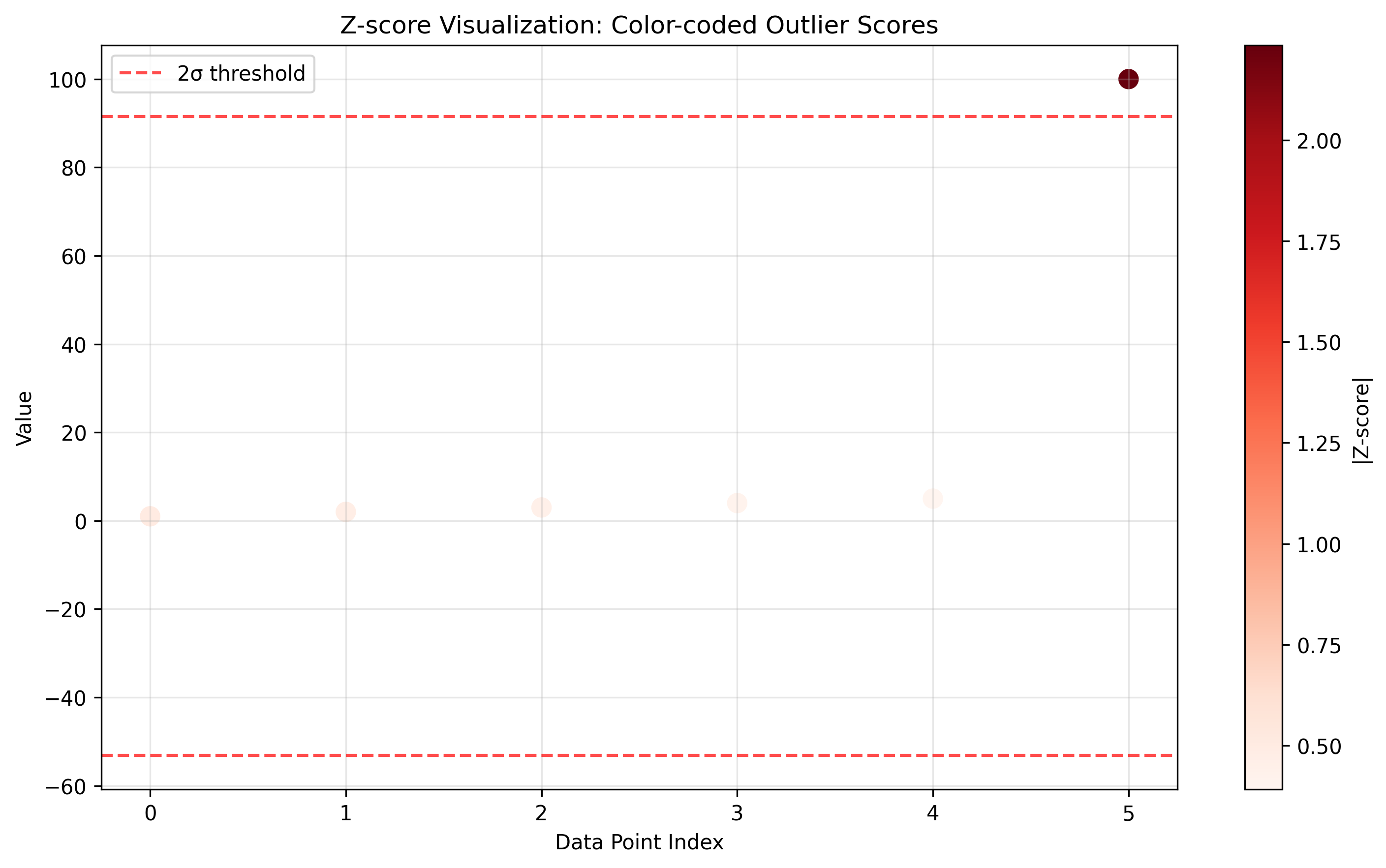
Density contour plot: Shows bivariate density with outliers highlighted
plt.scatter(normal_points[:, 0], normal_points[:, 1], label='Normal')
plt.scatter(outlier_points[:, 0], outlier_points[:, 1], color='red', label='Outliers')
plt.legend()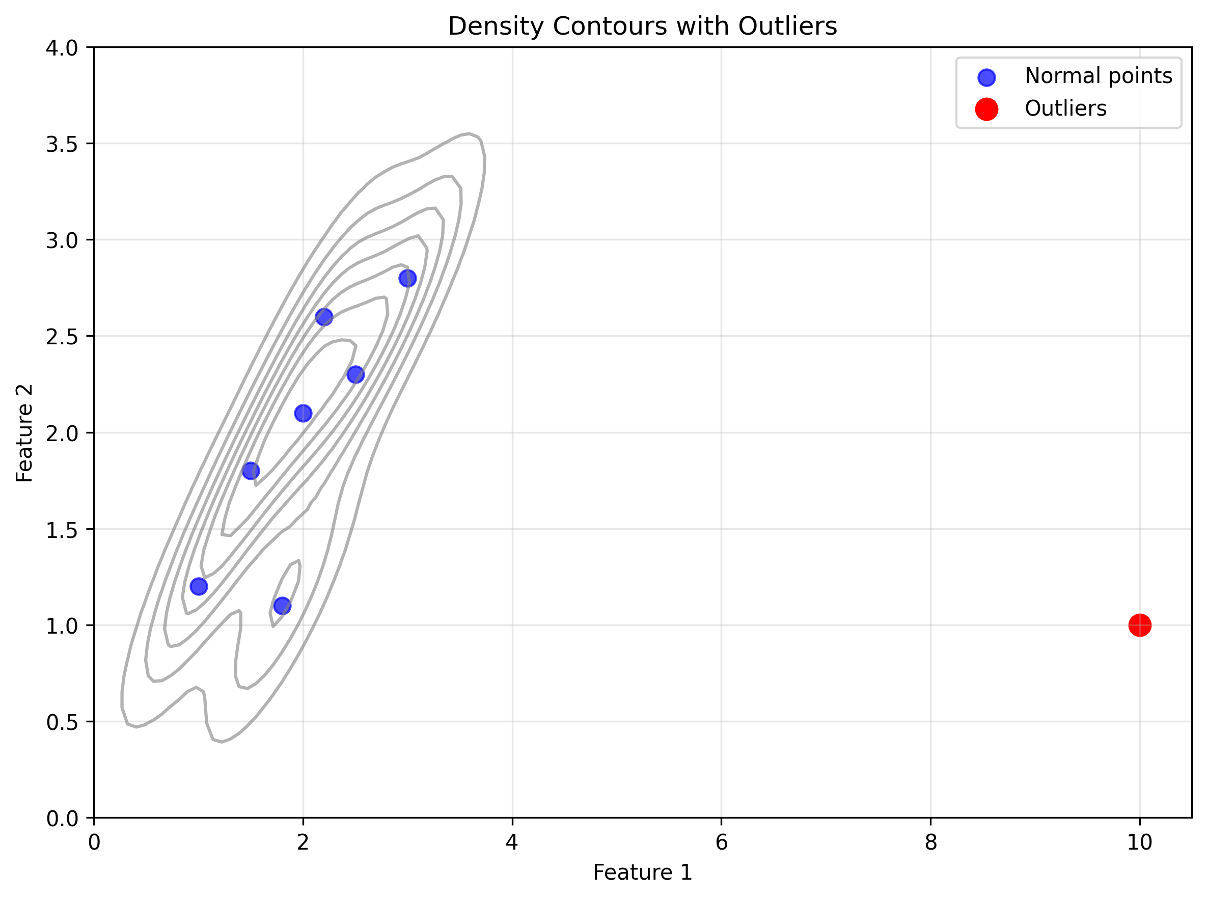
Anomaly detection methods can be categorized into three groups of methods:
Rules-based anomaly detection uses thresholds and logical conditions to identify outliers:
Univariate rules are simple threshold-based rules applied to single variables.
Range rules flag values outside expected ranges:
ages = [25, 30, -5, 150, 40]
outliers = [age for age in ages if age < 0 or age > 120]
print(f"Age outliers: {outliers}")
Age outliers: [-5, 150]Percentage rules flag extreme percentiles:
import numpy as np
data = np.array([10, 12, 15, 18, 20, 22, 25, 28, 30, 100])
outliers = data[data > np.percentile(data, 95)]
print(f"Top 5% outliers: {outliers}")
Top 5% outliers: [100]Business logic rules enforce domain-specific constraints:
employees = [{'salary': 80000, 'revenue': 70000}, {'salary': 50000, 'revenue': 200000}]
outliers = [emp for emp in employees if emp['salary'] > emp['revenue']]
print(f"Salary > revenue: {len(outliers)} employees")
Salary > revenue: 1 employeesMultivariate rules are combinations of univariate rules.
These can do things like check for consistency (that a start date is before an end date) or on ratios of features.
Combining multivariate rules is not straightforward, as the number of combinations grows exponentially with the number of features.
Statistical anomaly detection uses mathematical properties of data distributions to identify outliers.
These methods assume data follows certain statistical patterns and flag points that deviate significantly from these patterns:
The Z-score measures how many standard deviations a point is from the mean.
Points with an absolute Z-score greater than 2 or 3 are typically considered outliers.
Tradeoffs:
import numpy as np

data = np.array([1, 2, 3, 4, 5, 100])
mean = np.mean(data)
std = np.std(data)
z_scores = (data - mean) / std
outliers = data[np.abs(z_scores) > 2]The interquartile range (IQR) identifies outliers based on the spread of the middle 50% of the data.
Points outside one and a half times the IQR from the first and third quartiles are flagged as outliers.
Tradeoffs:
import numpy as np

data = [1, 2, 3, 4, 5, 100]
Q1, Q3 = np.percentile(data, [25, 75])
IQR = Q3 - Q1
outliers = [x for x in data if x < Q1 - 1.5*IQR or x > Q3 + 1.5*IQR]The Median Absolute Deviation (MAD) is a more robust alternative to standard deviation. It uses the median instead of the mean as a measurement of central expectation.
Tradeoffs:
import numpy as np

data = [1, 2, 3, 4, 5, 100]
median = np.median(data)
mad = np.median(np.abs(data - median))
outliers = [x for x in data if abs(x - median) > 3 * mad]The modified Z-score combines the interpretability of the Z-score with the robustness of MAD. It uses MAD instead of standard deviation for more robust outlier detection.
$$\text{Modified Z} = \frac{0.6745 \times (x - \text{median}(x))}{MAD}$$The constant 0.6745 makes MAD equivalent to standard deviation for normal distributions.
Tradeoffs:
import numpy as np

data = np.array([1, 2, 3, 4, 5, 100])
median = np.median(data)
mad = np.median(np.abs(data - median))
modified_z = 0.6745 * (data - median) / mad
outliers = data[np.abs(modified_z) > 3.5]Statistical scores can be combined across multiple features to create multivariate outlier detection:
Machine learning anomaly detection methods learn patterns from data. They can handle complex, multivariate relationships.
These algorithms are typically more sophisticated but less interpretable than rules or statistical methods.
We will look at a few different groups of machine learning methods:
Tradeoffs:
Identify outliers based on their distance to other points or clusters.
k-Nearest Neighbors (k-NN):
from sklearn.neighbors import NearestNeighbors
import numpy as np

knn = NearestNeighbors(
    # Number of neighbors to consider
    n_neighbors=5,
    # Algorithm selection (ball_tree, kd_tree, brute, auto)
    algorithm='auto',
    # Leaf size for tree algorithms
    leaf_size=30,
    # Distance metric
    metric='minkowski',
    # Power parameter for Minkowski metric (2=Euclidean)
    p=2
)

distances, indices = knn.fit(data).kneighbors(data)
anomaly_scores = distances.mean(axis=1)
Tradeoffs:
Identify outliers as points in low-density regions.
Local Outlier Factor (LOF):
from sklearn.neighbors import LocalOutlierFactor
import numpy as np

lof = LocalOutlierFactor(
    # Number of neighbors to consider
    n_neighbors=20,
    # Algorithm for neighbor search (auto, ball_tree, kd_tree, brute)
    algorithm='auto',
    # Leaf size for tree algorithms
    leaf_size=30,
    # Distance metric
    metric='minkowski',
    # Power parameter for Minkowski metric
    p=2
)

outlier_labels = lof.fit_predict(data)
anomaly_scores = -lof.negative_outlier_factor_
Kernel Density Estimation (KDE):
Tradeoffs:
Use clustering algorithms to identify outliers as points that don’t belong to any cluster or are far from cluster centers.
k-Means Outliers:
DBSCAN Outliers:
from sklearn.cluster import DBSCAN
import numpy as np

dbscan = DBSCAN(
    # Maximum distance between samples in same neighborhood
    eps=0.5,
    # Minimum samples in neighborhood to form core point
    min_samples=5,
    # Distance metric
    metric='euclidean',
    # Algorithm for neighbor search
    algorithm='auto',
    # Leaf size for tree algorithms
    leaf_size=30
)

cluster_labels = dbscan.fit_predict(data)
outliers = data[cluster_labels == -1]
Tradeoffs:
Isolation Forest:
from sklearn.ensemble import IsolationForest
import numpy as np

iforest = IsolationForest(
    # Number of base estimators in ensemble
    n_estimators=100,
    # Number of samples to draw to train each base estimator
    max_samples='auto',
    # Proportion of outliers in dataset
    contamination=0.1,
    # Number of features to draw to train each base estimator
    max_features=1.0,
    # Random state for reproducibility
    random_state=42
)

outlier_labels = iforest.fit_predict(data)
anomaly_scores = -iforest.score_samples(data)
Tradeoffs:
Gaussian Mixture Models (GMM):
One-Class SVM:
from sklearn.svm import OneClassSVM
import numpy as np

ocsvm = OneClassSVM(
    # Kernel type (linear, poly, rbf, sigmoid)
    kernel='rbf',
    # Kernel coefficient for rbf, poly, sigmoid
    gamma='scale',
    # Upper bound on fraction of outliers
    nu=0.1,
    # Regularization parameter
    C=1.0,
    # Degree for polynomial kernel
    degree=3
)

outlier_labels = ocsvm.fit_predict(data)
decision_scores = ocsvm.decision_function(data)
Tradeoffs:
Histogram-Based Outlier Score (HBOS):
from pyod.models.hbos import HBOS
import numpy as np

hbos = HBOS(
    # Number of histogram bins
    n_bins=10,
    # Regularization parameter for density estimation
    alpha=0.1,
    # Tolerance for histogram calculation
    tol=0.1,
    # Contamination proportion
    contamination=0.1
)

outlier_labels = hbos.fit_predict(data)
anomaly_scores = hbos.decision_scores_
Advantages:
Don’t expect zero anomalies in real data:
Separate different record types before applying anomaly detection:
# Separate analysis by transaction type
purchase_data = transactions[transactions['type'] == 'purchase']
sale_data = transactions[transactions['type'] == 'sale']

# Run anomaly detection on each separately
purchase_outliers = detect_anomalies(purchase_data)
sale_outliers = detect_anomalies(sale_data)
Ensemble approaches combine multiple anomaly detectors for improved performance:
Why use ensembles:
Ensemble strategies:
from pyod.models.combination import aom, moa, average
from pyod.models.iforest import IForest
from pyod.models.lof import LOF
from pyod.models.hbos import HBOS

# Train multiple detectors
clf1 = IForest(contamination=0.1)
clf2 = LOF(contamination=0.1)
clf3 = HBOS(contamination=0.1)

scores1 = clf1.fit(data).decision_scores_
scores2 = clf2.fit(data).decision_scores_
scores3 = clf3.fit(data).decision_scores_

# Combine scores using different method
avg_scores = average([scores1, scores2, scores3])
aom_scores = aom([scores1, scores2, scores3])
moa_scores = moa([scores1, scores2, scores3])
Tradeoffs:
Understanding why an anomaly detector flags records as outliers can be crucial for building trust and actionable insights.
The requirements for explanation vary significantly based on your audience and use case.
Interpretability generally refers to models that are inherently understandable, where you can directly see how decisions are made with minimal additional tools.
Explainability involves external techniques to understand anomaly detection labels and scores, often applied after the model has made predictions.
The distinction between interpretability and explainability exists on a spectrum rather than as rigid categories. Understanding this spectrum helps choose appropriate techniques for different audiences and use cases.
The spectrum in practice:
Gray areas and considerations:
Global explanations describe how the model works overall across the entire dataset.
Local explanations describe why a specific record was flagged as an anomaly.
These methods are inherently understandable without additional explanation tools:
Statistical methods:
Histogram-based methods:
Rules-based methods:
For complex models that lack inherent interpretability, use these post-hoc explanation methods.
Shows which features contribute most to anomaly detection globally:
from sklearn.inspection import permutation_importance
from pyod.models.iforest import IForest

# Train isolation forest
clf = IForest(contamination=0.1)
clf.fit(X_train)

# Calculate feature importance via permutation
perm_importance = permutation_importance(clf, X_test, scoring='roc_auc')
feature_names = ['age', 'salary', 'experience']

for i, importance in enumerate(perm_importance.importances_mean):
    print(f"{feature_names[i]}: {importance:.3f}")
age: 0.023
salary: 0.156
experience: 0.087Limitations: Feature importance doesn’t capture feature interactions or individual record explanations.
Provides both global and local explanations with theoretical guarantees:
import shap
from pyod.models.iforest import IForest

# Train model and get SHAP explainer
clf = IForest(contamination=0.1)
clf.fit(X_train)
explainer = shap.Explainer(clf.decision_function, X_train)

# Local explanation for specific record
shap_values = explainer(X_test[0:1])
print(f"Base value: {explainer.expected_value:.3f}")
print(f"SHAP values: {shap_values.values[0]}")
Base value: 0.102
SHAP values: [-0.025, 0.089, 0.034]Train simple, interpretable models to mimic complex model predictions:
from sklearn.tree import DecisionTreeClassifier, export_text
from pyod.models.iforest import IForest

# Complex model predictions
iforest = IForest(contamination=0.1)
complex_predictions = iforest.fit_predict(X)

# Simple proxy model
proxy = DecisionTreeClassifier(max_depth=3)
proxy.fit(X, complex_predictions)

# Proxy provides interpretable rules
rules = export_text(proxy, feature_names=['age', 'salary', 'experience'])
print(rules)
|--- salary <= 75000.00
| |--- age <= 25.00
| | |--- class: 0 (normal)
| |--- age > 25.00
| | |--- experience <= 2.00
| | | |--- class: 1 (anomaly)Partial Dependence Plots: Show how anomaly scores change with individual features:
from sklearn.inspection import PartialDependenceDisplay
import matplotlib.pyplot as plt

# Create partial dependence plot
PartialDependenceDisplay.from_estimator(clf, X, features=[0, 1], feature_names=['age', 'salary'])
plt.show()
Individual Conditional Expectation (ICE) plots: Show prediction changes for individual records across feature values.
Show minimum changes needed to change a prediction from anomaly to normal:
def generate_counterfactual(model, anomalous_record):
    """Find minimal changes to make record normal"""
    counterfactual = anomalous_record.copy()

    # Iteratively modify features with smallest changes
    for feature in features_by_importance:
        modified_record = counterfactual.copy()
        modified_record[feature] = find_normal_value(feature)

        if model.predict([modified_record])[0] == 0:  # Normal
            return modified_record, calculate_changes(anomalous_record, modified_record)

    return None

original = [25, 150000, 2]  # [age, salary, experience] - flagged as anomaly
counterfactual, changes = generate_counterfactual(model, original)
print(f"Change salary from {original[1]} to {counterfactual[1]} to be normal")
Change salary from 150000 to 80000 to be normalIn this lesson we’ve covered:
These techniques enable you to find interesting data, clean datasets, detect fraud, monitor systems, and identify rare events across diverse domains from finance to healthcare to cybersecurity.
Recommended resources:
